Forecasting power prices 24 hours ahead
Own day-ahead price models for four European power markets — period by period and day by day — built end to end from data ingestion to validation. This page shows the results and the method. The Spanish model is open: its code and daily forecasts are at prevision-precio-espana.
The result
Between 34% and 49% less error than the industry reference
The metric is mean absolute error (MAE) in euros per megawatt-hour, across every period of roughly 18 months the model never saw during training. Next to it, the reference any forecast in this market is measured against: repeating yesterday's price for the same hour, which is surprisingly hard to beat because power prices are strongly seasonal.
| Market | Model MAE | D-1 MAE | Improvement | Correlation | Error / mean price | Periods evaluated |
|---|---|---|---|---|---|---|
| Spain | 9.73 | 17.94 | 45.7% | 0.967 | 14.8% | 36,142 |
| Germany | 14.22 | 27.61 | 48.5% | 0.908 | 14.4% | 36,993 |
| France | 15.93 | 24.05 | 33.8% | 0.897 | 23.6% | 36,570 |
| Netherlands | 16.36 | 26.06 | 37.2% | 0.851 | 17.0% | 36,478 |
Evaluation windows between February 2025 and September 2026, each market with its own. Every figure comes from the validation described below, never from the training set.
On the unit: on 1 October 2025 the European market moved to 15-minute settlement periods instead of hours, so the model now predicts 96 prices per day where it used to predict 24. The data covers both regimes, and everything called a "period" here is an hour up to that date and a quarter-hour after it.
Two products, one model
The full-day block is a different market, and it forecasts far better
Someone buying power for a factory or hedging a portfolio does not always trade individual quarter-hours: they trade the full-day block, a product with its own liquidity and its own futures curve. That is a different question, and the project delivers it as a second product.
The interesting part is that no new model is needed. Four alternatives were tested — training a daily model from scratch, correcting the daily residual, a distilled model fed with the quarter-hourly predictions as inputs, and reweighting the ensemble against a daily objective — and all four lose to the simple option: averaging the day's 96 predictions. Averaging is itself a variance reduction that no new model manages to beat.
The result is a daily error between 24% and 37% lower than the single-period error, because averaging cancels the independent errors of each quarter-hour. In Spain it drops from 9.73 to 6.21 EUR/MWh.
| Market | Daily MAE | Naive daily MAE | Improvement | Correlation | Days evaluated |
|---|---|---|---|---|---|
| Spain | 6.21 | 13.84 | 55.1% | 0.977 | 327 |
| Germany | 10.78 | 22.53 | 52.2% | 0.905 | 319 |
| France | 10.36 | 18.42 | 43.8% | 0.941 | 325 |
| Netherlands | 11.07 | 20.30 | 45.5% | 0.833 | 320 |
The daily reference is the previous day's average. Only complete days are evaluated, so averages over truncated days are never mixed in.
How the model evolved
From a model you can understand to one that gets it right
This project did not start with trees and neural nets. It started at the opposite end: rebuilding the price from the market's real economics, with a model you could sketch on a napkin. That model was fully understandable and missed by too much.
What follows is a chain of decisions of the same kind, taken one at a time: add a layer of complexity that lowers the error and, in exchange, takes away a piece of the explanation. Each step was only taken after measuring what it bought, because a component you cannot explain and have not measured either is not a model, it is a superstition.
At each step, the two currencies of the trade: the mean error in Spain (MAE, in EUR/MWh, over the same window of 36,142 periods) and how much of the result can be explained without ending at "the model says so".
-
00
The starting point: repeat yesterday's price
The reference any forecast in this market is compared against. It is not a model and it is still hard to beat, because the power price is strongly seasonal. It is fully understandable: today's number is yesterday's at the same hour. Everything that follows is measured against this line.
17.94 MAE Explainable ●●●●●
-
01
Before any model, the data
Thirty-eight sources pulled from their official origin, audited one by one against their documentation, and a filter that keeps out anything not published before the auction closed. This is the only layer of the whole path that costs no understanding: it provides it. A complex model on dirty data is not more powerful, it just learns the dirt faster.
- 38 sources
- 33 automated audits
- History from 2023
- Only information available on D-1
— no forecast yet Explainable ●●●●●
-
02
Rebuild the price from the mechanism
A simulator that stacks the marginal cost of each technology against demand, the same way the market clears. It is the most explainable model you can build here: every euro has a physical cause you can point at. And it falls short — a correlation of 0.520, not enough for production. This is the decision that orders everything else: if you want production-grade error, you have to start paying in understanding. What it did leave behind, and what justifies it, is knowing which variables matter and why.
0.520 correlation · dropped from production Explainable ●●●●●
-
03
First trade: trees on those variables
Gradient boosting on what the simulator taught, in two splits of the same data: one with all hours pooled, which uses the whole history, and one with a model per hour of the day, because 3 a.m. and 8 p.m. are almost different markets. The error falls from 17.94 to 10.34. In exchange there is no equation any more, there are learned rules: you can still ask which variables carry weight, but no longer why this particular hour.
10.34 MAE · −42% vs the reference Explainable ●●●○○
-
04
Split the problem: the zero-price gate
The power price is not a continuous variable: it has a floor with concentrated mass — 6.3% of periods land exactly there — and a regressor trained across the whole range spends its life splitting the difference between two distinct regimes. The fix is a classifier that decides the regime before predicting the number. There is no longer one model: there is one that decides and one that predicts. It is the component that buys the most, and it is not the most sophisticated one.
10.20 MAE · −0.14 Explainable ●●○○○
-
05
Crossing the line: adding something you cannot read
A neural net as the third ensemble member. It is not there to try something modern, it is there for a mechanical reason: a tree model cannot extrapolate. It averages leaves, so it never predicts above the maximum it saw in training — exactly the failure at price spikes. A network can step outside that range. It was accepted because it was measured where it wins: across the most expensive 5% of hours, the third member, the calibration and margen_neto together take the error from 14.03 to 10.46.
9.81 MAE · from 10.20 Explainable ●○○○○
-
06
The last layer no longer talks about the market
The high-tail calibration corrects a bias that does not come from electricity, but from the mismatch between training and evaluation: the models minimise squared error, whose optimum is the mean, but are scored on absolute error, whose optimum is the median, so they shrink towards the centre and fall short at the top. It is a pure statistical artefact: explaining it says nothing about the market. It is worth 0.07 EUR/MWh, and by here there is nothing left to teach about the price.
- Quantile regression · Spain
- Log scale + Duan · Germany and the Netherlands
9.80 MAE · −0.01 Explainable ○○○○○
-
07
Where the understanding comes back
The explanation is not lost: it moves. Instead of being read inside the model, it is measured from outside. Every component was evaluated separately over the same window of 36,142 periods, with walk-forward validation, its confidence interval resampling whole months, and the whole thing recomputed without the month that contributes most. Then it was checked whether the gain came from where it was supposed to. An opaque model whose contribution is measured piece by piece is better understood than a transparent one that was never validated.
9.73 MAE · 0.967 correlation · −45.7% vs the reference Auditable ●●●●●
That is the whole path: from 17.94 to 9.73 EUR/MWh (9.80 with these four components; 9.73 today, with `margen_neto` added later, see below), and from a model you could describe in one sentence to one you can only audit by measuring. It is not an accident, nor a race to use the newest technique: it is a sequence of explicit trades, each with its number beside it.
That is also why everything tried is written down, whether it worked or not: the project carries 144 numbered technical findings, a good share of them discarded experiments with the reason they were discarded. Layers that did not buy enough never went in.
The Spanish model · the main line
Every component had to earn its place, and you can see what each one bought
Spain is the market with the most time invested and the best result: 9.73 EUR/MWh of mean error against a mean price of 65.61, with a correlation of 0.967. It is not one model but five components stacked on top of each other, and each was adopted only after measuring separately how much error it removed.
The chart below is measured over the same window of 36,142 periods in all five versions, which is the only way the differences mean anything.
The component that contributes most is not the most sophisticated one. The zero-price gate is a classifier that decides, before predicting a number at all, whether an hour will settle at zero or below. It exists because power prices are not a continuous variable: they have a floor with concentrated mass — 6.3% of periods land exactly there — and a regressor trained across the whole range spends its life splitting the difference between two distinct regimes.
And where the stack really shows is in the expensive hours, which are the ones that cost money:
Model families
Each part of the problem calls for a different tool
The day-ahead price is not one statistical problem: it is a zero-price regime, a fairly smooth central body, and an upper tail with few examples and a lot of money at stake. Using a single model for all three is what caps most attempts. These are the families that ended up in production, and why each one is where it is.
The body of the model. Two members from the same family but with a different split of the data: one trained across all hours at once, the other a separate model per hour of the day. The first exploits the full history; the second captures that 3 a.m. and 8 p.m. are almost different markets.
The third member, and it is there for a mechanical reason rather than novelty: a tree model cannot extrapolate. It averages leaves, so it never predicts above the maximum it saw in training — exactly the failure mode in price spikes. A network can leave that range, and it shows precisely there.
Separates the regime before predicting a number. It treats the price floor as what it is — a concentrated mass of probability, not the tail of a continuous distribution — and lets the regressor handle only the positive side.
Corrects a bias that comes from the mismatch between training and evaluation: the models minimise squared error, whose optimum is the mean, but are scored on absolute error, whose optimum is the median. The result is shrinkage towards the centre and under-prediction at the top. A line to the median is fitted and applied only above a threshold.
The same problem solved from the other side, adopted in Germany and the Netherlands: instead of correcting the output, change the scale on which error is measured during training, so that a single 600 EUR/MWh hour does not dominate the fit. It is the only change that improved the model's ability to rank expensive hours against each other.
Members are blended with weights chosen month by month over a grid search, always using months already observed and never the period being evaluated. A small detail that separates a real result from an inflated one.
Before all of the above, a model that is not statistical: it stacks the marginal cost of each technology against demand to rebuild the price from the actual economic mechanism. It reaches a correlation of 0.520 — not enough for production, but it is what taught which variables matter and why.
Good practice
The number is only worth something if the validation is honest
In time series it is very easy to produce an excellent and false figure: all it takes is letting in, unintentionally, a piece of data that did not yet exist at the moment of prediction. The whole design is built around preventing that.
-
01
Training uses only the past
Monthly walk-forward validation: to predict a month, the model is trained only on the preceding ones and retrained as it advances. There is never a random split, which in a time series lets the model see the future.
-
02
Only data available at D-1 gets in
Every variable passes a prior filter: was it published before gate closure? Actual generation, imbalances and balancing prices are known afterwards, so they serve as diagnostics and stay out of the model.
-
03
Everything estimated is estimated on the past
Not just the model: thresholds, calibrations and the weights that blend the members too. Any constant tuned by looking at the test period contaminates the result.
-
04
Comparison is against the stored previous version
Each improvement is measured against the production model's predictions already written to disk, not against a stand-in retrained for the occasion. That way the comparison isolates the change being tested.
-
05
Check whether the gain is real or just a good month
The aggregate comes with a confidence interval — resampling whole months, because errors in consecutive hours are correlated — and is recomputed after dropping the single best month. A gain that collapses when one month is removed was not a gain.
-
06
Check that the gain comes from where it was supposed to
If a component exists to fix expensive hours, the gain has to concentrate in months with expensive hours. When it does not, the change is still adopted — error is the criterion — but it is written down that the mechanism was something else, and that steers the next piece of work.
Everything tried is documented, whether it worked or not: the project holds 144 numbered technical findings, and a good share of them are discarded experiments with the reason they were discarded. That is what stops the same dead end being walked into again three weeks later.
Diagnosis
The error is not spread evenly: it lives in the extremes
An aggregate MAE hides where it comes from. Splitting periods by the price they ended up settling at reveals the real shape of the problem — and shows that each market fails somewhere different.
Spain is the flattest market: its worst band (11.26) barely exceeds its best (10.06), and the zero-price regime is almost entirely solved (2.08). The other three have their error concentrated in the extremes.
The other three markets
Each market is its own project, not the same model translated
What works in Spain is an idea to test in Germany, not a conclusion to carry over. Degree days help in France and in none of the other three; the tail calibration was adopted in Spain and France and dropped in Germany and the Netherlands after being measured. The only improvement that has travelled intact is the log scale on the training target.
The clearest example of why each market has to be studied separately is German, and it is a subsidy rule.
A clause in German renewables law draws the shape of negative prices
The German renewables act (EEG §51) suspends an installation's market premium when the price is negative for several consecutive hours, and that threshold has been tightened three times since 2023 — from six hours down to every quarter-hour. If the rule is what drives behaviour, the price should not simply be "negative": it should sink deeper the longer the run lasts, then recover once installations have already lost the premium and no longer have a reason to bid low.
That is exactly what shows up across 1,795 negative German hours. And the trough is 60% deeper since the February 2025 reform.
The German market has shifted underneath the model
A model trained on three years of history implicitly assumes the market of three years ago resembles today's. In Germany that has stopped being true, and it can be quantified.
| Indicator | 2023 | 2026 |
|---|---|---|
| Hours with low residual load (< 5 GW) | 2.9% | 13.1% |
| Solar capture rate | 0.758 | 0.515 |
| Wind capture rate | 0.839 | 0.908 |
| Median hour of prices > 200 EUR/MWh | 17:00 | 20:00 |
The capture rate is the average price a technology earns divided by the market's average price. Solar has gone from earning 76% of the average price to 51%: it cannibalises itself by concentrating all its output in the same hours. Wind, spread across the day, has improved. And the price peak has moved three hours later into the evening with 10 GW less residual load: today's expensive hours are summer evenings that any rule based on demand level would classify as comfortable.
Four market studies
The same data platform answers questions that are not about forecasting
Valuation and market-structure studies were built on the same infrastructure. Each with its design written before any results were seen, its own model, and a record of what it failed to confirm. Here are four.
A gas plant loses money on average and is still worth money
Valuing a gas plant by its average margin — the power price minus its cost to run, hour by hour — gives −20.78 EUR/MWh: it would lose money if forced to run all 24 hours. But it is not forced to. It runs only when it pays, and that right to choose is what gets valued: +8.92 EUR/MWh.
The gap, 29.70 EUR/MWh, is the value of optionality, and it is why a plant is not a contract but an option. It exercises 38.7% of hours.
What the annual series shows is more interesting still. The average margin collapses — from −11.34 to −40.78 EUR/MWh in four years, from the price erosion renewables bring — but the option value barely moves, between 7.99 and 9.47. The plant exercises less and less often (from 47% to 28% of hours) and those hours stay almost as profitable. The more variable renewables enter, the more flexibility is worth and the less baseload generation is.
The figure above is an upper bound: it assumes switching on and off hour by hour at no cost. Under a realistic dispatch — minimum 4 hours on, 2 hours off and 50 EUR/MW per start, solved by dynamic programming — the value falls to 7.37 EUR/MWh, only 17% lower. The reason is that profitable hours are not scattered: they come in blocks, so the minimum run-time rarely forces the plant to stay on through bad hours.
Access to more markets is worth far more to a small battery
A battery makes money buying low and selling high. The study asks how much is added by also trading the continuous intraday market rather than day-ahead alone, and whether that depends on battery size.
It does, enormously. With an optimised dispatch and real technical constraints, adding intraday more than doubles the revenue of a 1-hour battery (+126%), but lifts a 4-hour one by only 40.6%.
The mechanism is clear: a 4-hour battery already captures the day's big spread from day-ahead alone, so intraday adds little. A 1-hour battery cannot do that and lives on finding many small opportunities — exactly what a continuous market offers. It is a concrete commercial conclusion: revenue stacking matters far more the shorter the battery.
The French interconnector is congested far more than it looks
Spain and France share a single power corridor. When it has spare capacity the two prices converge; when it saturates, they separate. The difference between them — the basis — averages just −1.02 EUR/MWh, and that figure is misleading: its standard deviation is 39.75.
Broken down: only 33% of hours have the two markets effectively coupled, while 41.2% show strong decoupling, above 20 EUR/MWh. The interconnector is an active constraint most of the time, not an occasional exception.
And my favourite finding here is methodological. French nuclear unavailability appeared to explain nothing: its same-instant correlation with the basis is +0.07, near zero and with the opposite sign to theory. But running a Granger causality test across lags, it appears strongly from 6 hours onwards. A weak contemporaneous correlation does not rule out a real relationship — you may simply be looking at the wrong moment.
With the three variables together, a tree model cuts the basis prediction error from 24.19 to 21.43 EUR/MWh against predicting the mean, and Spanish wind dominates feature importance. But to classify whether congestion will occur, a simple threshold on interconnector utilisation (F1 0.661) beats the full model (0.641). Where a dominant structural driver exists, extra complexity buys nothing.
A battery earns more by standing ready than by moving energy
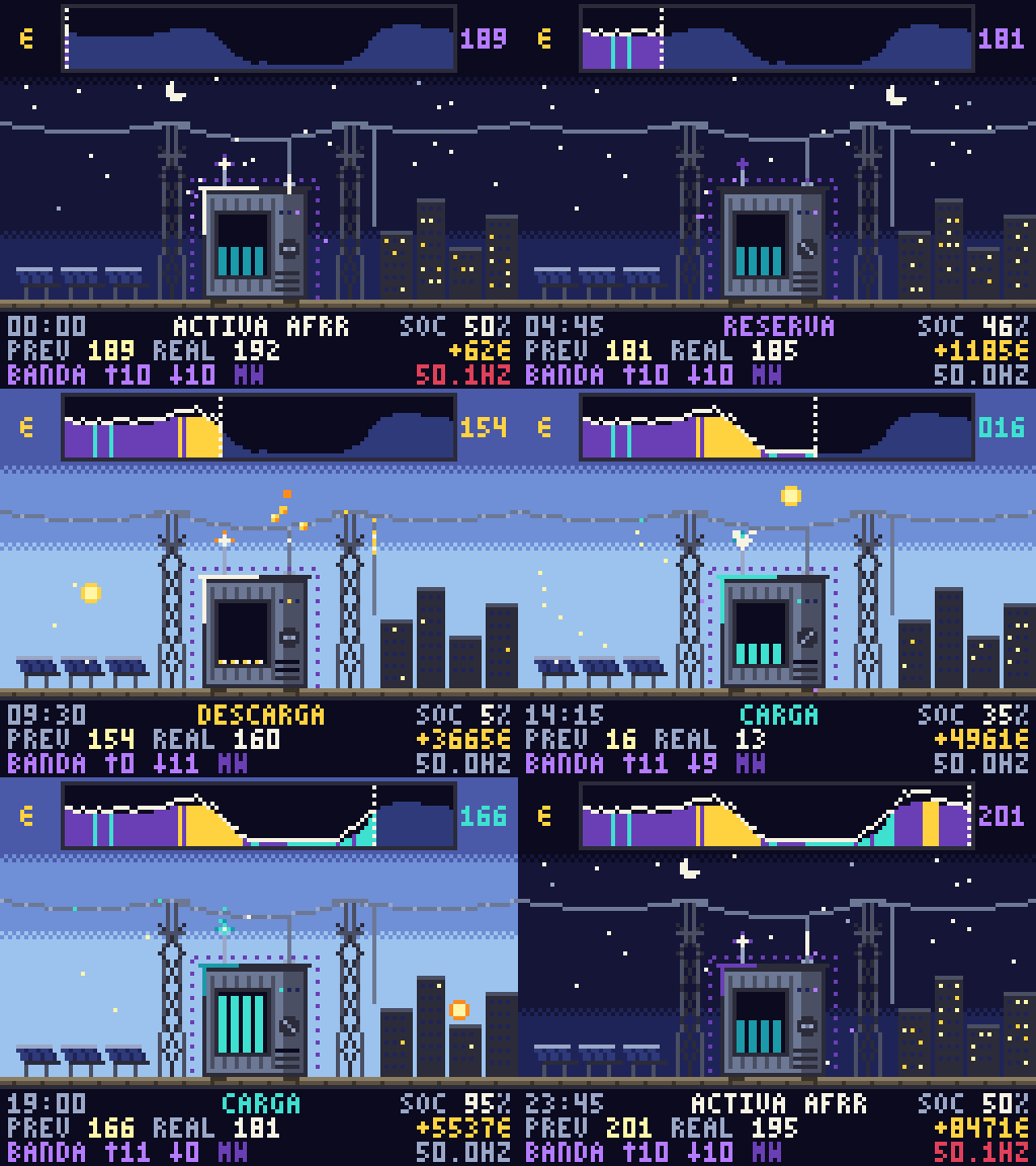
A 20 MWh / 10 MW battery that only arbitrages the day-ahead market —charging in the solar trough, selling at the peaks— nets EUR 687,552 over 531 days, after degradation. If it also reserves capacity for Spain's secondary frequency regulation (the aFRR band), the net rises to EUR 1.59 million: being available pays more than moving energy.
When the grid operator uses that reserve, the activated energy is paid separately and at far better prices than day-ahead. Counting it, the net reaches EUR 1.99 million, about EUR 137,000 per MW per year. All with a causal backtest: dispatch is decided with the model's forecast before the auction closes and settled at the real price.
The animation replays a real day, 10 September 2026, quarter-hour by quarter-hour. Interactive version.
The data
Thirty-eight sources, ingested and audited one by one
There is no ready-made dataset behind this. Each source is pulled from its official origin, checked against the documentation — time zones, units, resolution changes, later revisions — and passes an audit before it enters any model. History starts in 2023 and updates daily.
Scope
What this page shows and what it does not
This page shows results and method: what was measured, how it was validated, and what was learned about the market along the way. The figures are internally reproducible and come straight from the project's validation artefacts.
The code, the engineered features and the trained models are not published. I am glad to walk through them in detail in a conversation, and can demonstrate the project running live.